Introduction

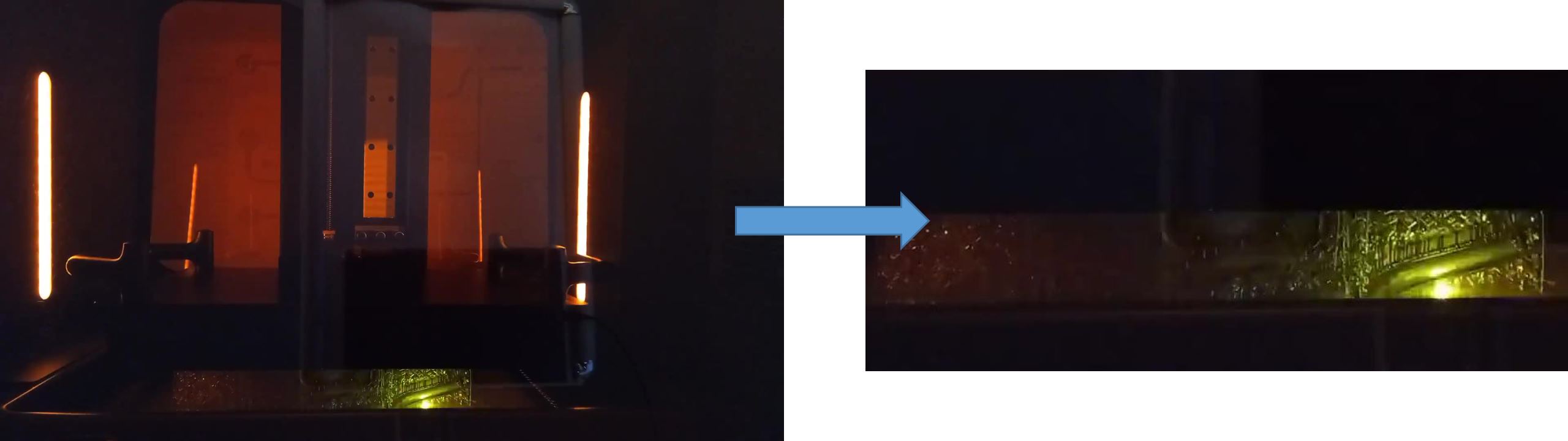
I wanted to record a time lapse of a SLA 3D printer (Formlabs Form 3L) to show the object coming to life. For other printers one can inject gcode to synchronize the shots and get a clean time lapse, unfortunately this printer use proprietary software to control the print so it is not possible. I then decided to use an android tablet and a dedicated app from the store. The result is quite cool as the material used is transparent so you can see the laser that hits the resin. As you can see one of the main issues is that the cover of the printer is highly reflective and you can see what is in front of it. I will have to try again with a polarizing filter to see if that reduce the issue.

The second issue is that for each layer, the printer raises and lowers the object to mix the resin. This is quite annoying as it breaks the flow of the object being built taking up about half of the video time. Instead, I would like to see just the object slowly growing layer after layer without intermissions.

Editing the video removing the snippets by hand is quite impossible, as the object is composed by thousands of layers.

Being the video quite repetitive, I thought I could use machine learning to automatically identify the frames that I want and get rid of the ones I don't want.

Frames Extraction

The first step is to extract all frames into single images, since I don't think working directly on the video is really feasible. To do so I used ffmpeg.

The command template is the following:

ffmpeg -i <input path> -qscale:v <quality> <output path>%05d.jpg

The %05d part tells ffmpeg to add an incremental number at the end of the file name, padded to five digits (e.g: 00001.jpg). You can adapt the number as required, I had around 21000 frames so 5 digits is the correct number.

The quality parameter indicates the quality of the output, depending from the encoder (in this case the jpeg quality) and goes from 1 (highest quality) to 31 (lowest quality). You can omit this parameter.

Here's the full command I used:

ffmpeg -i input.mp4 -qscale:v 2 frames/frame_%04d.jpg

Note: you have to create the "frames" directory before launching the command, otherwise it will fail.

Images Preparation

An issue that I encountered is that with Full HD images (1920x1080), the code would crash after a while due to high RAM usage.

I can see 3 solutions:

• Get more RAM (use a dedicated service on cloud)
• Reduce the images size (scale down the images)
• Crop the images

Obviously the first option would be the one that require less work, but I chose to crop the images so that I can also get the benefit of a video with just the object and not the whole printer, reducing also some "noise". Once we have the final set of images that we want to keep we can then still apply the same selection to the original images getting the complete Full HD video.

Images Reduction

To crop all the images in batch I used the software Irfranview. If this is not suitable for you, you can find more alternatives searching for "batch crop images" or "bulk crop images". I'm sure you can do it directly in code but using a dedicated software was quicker for me.

Setup of Training Images

Once we have a set of images that our hardware can finally support, we can start preparing a set of images for training our machine learning model.

To do so, I just selected some sequences of images from the whole to tag them manually. I choose around 1000 images from different point of the video (so that the object is in different phases of printing) but I think that a lower number of images would work as well, since we only have 2 classes to identify: images where the laser is on and images where the printer is mixing the resin.

I copied the selected images in a "training" folder and manually divided them between 2 subfolders: "OK" and "KO". This can seem a lot of work to do manually but I could easily identify them by the thumbnail end move dozens of images at a time.

Coding

We are now ready to start build our machine learning model, but first let's prepare our environment.

Environment Setup

First of all we need python (3). To keep our configuration clean we can create a dedicated environment. Create a directory for the code, use the shell to move into it and launch this command:

python -m venv .

This will create a dedicated virtual environment that is isolated from our main python configuration. We then need to activate the environment running the dedicated script (see the reference documentation to get the command for your OS).

In PowerShell:

.\Scripts\Activate.ps1

We can then proceed to install the required libraries.

pip install matplotlib numpy tensorflow pathlib shutil

Training

The code I used is based on the Tensorflow Image Classification tutorial. You can check it for more details.

Start by importing the libraries:

import matplotlib.pyplot as plt
import numpy as np
import tensorflow as tf

from tensorflow import keras
from tensorflow.keras import layers
from tensorflow.keras.models import Sequential

import pathlib

We can then configure the images details:

batch_size = 32
img_height = 330
img_width = 770

train_dir = pathlib.Path("training")

We can then create the training and validation sets, in this case 80% of the previously classified images are used for training and 20% for validation (according to the validation_split parameter).

train_ds = tf.keras.utils.image_dataset_from_directory(
  train_dir,
  validation_split=0.2,
  subset="training",
  seed=123,
  image_size=(img_height, img_width),
  batch_size=batch_size)

val_ds = tf.keras.utils.image_dataset_from_directory(
  train_dir,
  validation_split=0.2,
  subset="validation",
  seed=123,
  image_size=(img_height, img_width),
  batch_size=batch_size)

The class names are directly inferred from the directory names. We can verify that with the following lines (you can omit the print but we will need the variables later):

class_names = train_ds.class_names
print(class_names)
num_classes = len(class_names)

The output should report "OK" and "KO": the folder names that we previously used to classify the images.

We can then setup the buffering and normalize the data values (again, check the official tutorial for details).

AUTOTUNE = tf.data.AUTOTUNE

train_ds = train_ds.cache().shuffle(1000).prefetch(buffer_size=AUTOTUNE)
val_ds = val_ds.cache().prefetch(buffer_size=AUTOTUNE)

normalization_layer = layers.Rescaling(1./255)

normalized_ds = train_ds.map(lambda x, y: (normalization_layer(x), y))
image_batch, labels_batch = next(iter(normalized_ds))

Now we can instantiate our model:

model = Sequential([
  layers.Rescaling(1./255, input_shape=(img_height, img_width, 3)),
  layers.Conv2D(16, 3, padding='same', activation='relu'),
  layers.MaxPooling2D(),
  layers.Conv2D(32, 3, padding='same', activation='relu'),
  layers.MaxPooling2D(),
  layers.Conv2D(64, 3, padding='same', activation='relu'),
  layers.MaxPooling2D(),
  layers.Flatten(),
  layers.Dense(128, activation='relu'),
  layers.Dense(num_classes)
])

model.compile(optimizer='adam',
              loss=tf.keras.losses.SparseCategoricalCrossentropy(from_logits=True),
              metrics=['accuracy'])

model.summary()

We can then finally train out model.

epochs=3
history = model.fit(
  train_ds,
  validation_data=val_ds,
  epochs=epochs
)

You can play with the number of epochs, in my case 3 was enough (the more epochs, the more time it takes to run). To get a better ideas of how the model performs after each training epoch you can plot some chart:

acc = history.history['accuracy']
val_acc = history.history['val_accuracy']

loss = history.history['loss']
val_loss = history.history['val_loss']

epochs_range = range(epochs)

plt.figure(figsize=(8, 8))
plt.subplot(1, 2, 1)
plt.plot(epochs_range, acc, label='Training Accuracy')
plt.plot(epochs_range, val_acc, label='Validation Accuracy')
plt.legend(loc='lower right')
plt.title('Training and Validation Accuracy')

plt.subplot(1, 2, 2)
plt.plot(epochs_range, loss, label='Training Loss')
plt.plot(epochs_range, val_loss, label='Validation Loss')
plt.legend(loc='upper right')
plt.title('Training and Validation Loss')
plt.show()

When you are satisfied, you can save the model for further analysis, without the need of other training rounds.

model.save('saved_model/my_model')

We can then create a separate script for classification. Just copy the library imports and configuration, and add:

import shutil

data_dir = pathlib.Path("data")
out_dir = pathlib.Path("output")

data_list = list(data_dir.glob('*'))

The data directory contains all the original (cropped) images, while the output directory is the one that will contains the filtered images.

We can then load the model that we previously saved:

model = tf.keras.models.load_model('saved_model/my_model')

model.summary()

class_names = ('KO', 'OK')

We can then loop through all the images to classify them:

for filename in data_list:
  print(filename)
  img = tf.keras.utils.load_img(
    filename, target_size=(img_height, img_width)
  )
  img_array = tf.keras.utils.img_to_array(img)
  img_array = tf.expand_dims(img_array, 0) # Create a batch

  predictions = model.predict(img_array)
  score = tf.nn.softmax(predictions[0])

  print("This image most likely belongs to {} with a {:.2f} percent confidence.".format(class_names[np.argmax(score)], 100 * np.max(score)))

  if predictions[0][1] > 0.5:
    print('!!!!!!!!! OK !!!!!!!!!')
    shutil.copy(filename, out_dir)

Here, if the image is one that we want, we copy it to the output directory keeping the original file name. At the end of the loop, if everything worked correctly, we have our output directory containing all the images we want!

We can then proceed to join back the images in a single video!

If we want to use ffmpeg (I guess this can be also done with other higher-level software), there is still a problem, as ffmpeg requires that all file names have a sequential numbering without gaps in it, and since we removed more than half of the images we surely have lots of missing numbers (there are also ways to give ffmpeg the exact list of files but didn't work for me).

We could easily fix this directly in the classification code, but I choose to make another copy of the files to keep the original filenames.

For this I created another small script that just takes all files and renames them keeping a sequential numbering.

import pathlib
import shutil

out_dir = pathlib.Path("output")
data_list = list(out_dir.glob('*'))

index = 0
for filename in data_list:
  new_filename = f'filtered/frame_{index:05d}.jpg'
  index = index + 1
  shutil.copy(filename, new_filename)

Now we should have our renamed files in the "filtered" directory.

The last step is to run ffmpeg to encode the final video:

ffmpeg -i frame_%05d.jpg -c:v libx264 final_output.mp4

And there you have it!

Warning: flashing lights!

This video was furtherly sped up and edited with the addition of a final clip of the object lifted up.

The following is the full-size and normal speed version,